রোডম্যাপ / ফেজ ৯ · Reinforcement Learning
Proximal Policy Optimization (PPO)
A2C throws away each rollout after one update. PPO wraps the policy gradient in a clipped importance ratio so you can do 10+ epochs on the same data without the policy exploding. Schulman et al. (2017). Still the default policy-gradient algorithm in 2026.
Type: Build Languages: Python Prerequisites: Phase 9 · 06 (REINFORCE), Phase 9 · 07 (Actor-Critic) Time: ~75 minutes
The Problem
A2C (Lesson 07) is on-policy: the gradient requires data sampled from the current . Take one update, and changes; the data you used is now off-policy. Re-use it and your gradient is biased.
Rollouts are expensive. On Atari, one rollout across 8 envs × 128 steps = 1024 transitions and a dozen seconds of environment time. Throwing that away after one gradient step is wasteful.
Trust Region Policy Optimization (TRPO, Schulman 2015) was the first fix: constrain each update so the KL divergence between old and new policy stays below . Theoretically clean, but requires a conjugate-gradient solve per update. Nobody runs TRPO in 2026.
PPO (Schulman et al. 2017) replaces the hard trust-region constraint with a simple clipped objective. One extra line of code. Ten epochs per rollout. No conjugate gradients. Good-enough theoretical guarantees. Nine years later it is still the default policy-gradient algorithm for everything from MuJoCo to RLHF.
The Concept
The importance ratio.
This is the likelihood ratio of the new policy vs the policy that collected the data. means no change. means the new policy is twice as likely to take as the old.
The clipped surrogate.
Two terms:
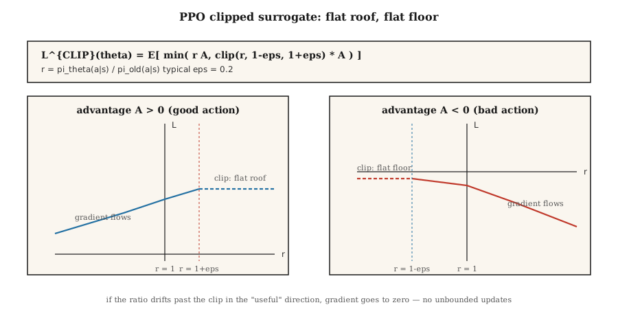
- If the advantage and the ratio tries to grow past , the clip flattens the gradient — don't push a good action further than above old probability.
- If the advantage and the ratio tries to fall below (meaning we would make a bad action much less likely than the old policy did), the clip flattens the gradient: don't push a bad action further than below old probability.
The min handles the other direction: if the ratio has moved in the beneficial direction, you still get the gradient (no clipping on the side that would hurt you).
Typical . Plot the objective as a function of : a piecewise-linear function with a flat roof on the "good side" and a flat floor on the "bad side."
The full PPO loss.
Same actor-critic structure as A2C. Three coefficients, usually , , .
The training loop.
- Collect transitions across parallel envs for steps each.
- Compute advantages (GAE), freeze them as constants.
- Freeze as a snapshot of current .
- For epochs, for each minibatch of
(s, a, A, V_target, log π_old(a|s)):- Compute .
- Apply + value loss + entropy.
- Gradient step.
- Discard the rollout. Return to step 1.
and minibatches of 64 is a standard hyperparameter set. PPO is robust: the exact numbers rarely matter within ±50%.
KL-penalty variant. The original paper proposed an alternative using an adaptive KL penalty: with adjusted based on observed KL. The clipping version became dominant; the KL variant survives in RLHF (where KL to the reference policy is a separate constraint you always want anyway).
Interactive figure “ppo-clip”: open it on the curriculum site ↗
Build It
Step 1: capture log π_old(a | s) at rollout time
for step in range(T):
    probs = softmax(logits(theta, state_features(s)))
    a = sample(probs, rng)
    s_next, r, done = env.step(s, a)
    buffer.append({
        "s": s, "a": a, "r": r, "done": done,
        "v_old": value(w, state_features(s)),
        "log_pi_old": log(probs[a] + 1e-12),
    })
    s = s_next
The snapshot is taken once, at rollout time. It does not change during the update epochs.
Step 2: compute GAE advantages (Lesson 07)
Same as A2C. Normalize across the batch.
Step 3: clipped surrogate update
for _ in range(K_EPOCHS):
    for mb in minibatches(buffer, size=64):
        for rec in mb:
            x = state_features(rec["s"])
            probs = softmax(logits(theta, x))
            logp = log(probs[rec["a"]] + 1e-12)
            ratio = exp(logp - rec["log_pi_old"])
            adv = rec["advantage"]
            surrogate = min(
                ratio * adv,
                clamp(ratio, 1 - EPS, 1 + EPS) * adv,
            )
            # backprop -surrogate, add value loss, subtract entropy
            grad_logpi = onehot(rec["a"]) - probs
            if (adv > 0 and ratio >= 1 + EPS) or (adv < 0 and ratio <= 1 - EPS):
                pg_grad = 0.0  # clipped
            else:
                pg_grad = ratio * adv
            for i in range(N_ACTIONS):
                for j in range(N_FEAT):
                    theta[i][j] += LR * pg_grad * grad_logpi[i] * x[j]
The "clipped → zero gradient" pattern is the heart of PPO. If the new policy has already drifted too far in the beneficial direction, the update stops.
Step 4: value and entropy
Add standard MSE to the critic target and an entropy bonus on the actor, same as A2C.
Step 5: diagnostics
Three things to watch every update:
- Mean KL . Should stay in
[0, 0.02]. If it blows past0.1, reduceK_EPOCHSorLR. - Clip fraction — the fraction of samples whose ratio lies outside . Should be
~0.1-0.3. If~0, the clip never triggers → raiseLRorK_EPOCHS. If~0.5+, you are over-fitting the rollout → lower them. - Explained variance . Critic quality metric. Should climb toward 1 as the critic learns.
Pitfalls
- Clip coefficient mistuned. is the de-facto standard. Going to
0.1makes updates too timid;0.3+invites instability. - Too many epochs. routinely destabilizes because the policy drifts far from . Cap epochs, especially for large networks.
- No reward normalization. Large reward scales eat into the clip range. Normalize rewards (running std) before computing advantages.
- Forgetting advantage normalization. Per-batch zero-mean/unit-std normalization is standard. Skipping it wrecks PPO on most benchmarks.
- Learning rate not decayed. PPO benefits from linear LR decay to zero. Constant LR is often worse.
- Importance ratio math errors. Always
exp(log_new - log_old)for numerical stability, notnew / old. - Wrong gradient sign. Maximize the surrogate = minimize . A flipped sign is the most common PPO bug.
Use It
PPO is 2026's default RL algorithm across a surprising number of domains:
| Use case | PPO variant |
|---|---|
| MuJoCo / robotics control | PPO with Gaussian policy, GAE(0.95) |
| Atari / discrete games | PPO with categorical policy, rolling 128-step rollouts |
| RLHF for LLMs | PPO with KL penalty to reference model, reward from RM at end of response |
| Large-scale game agents | IMPALA + PPO (AlphaStar, OpenAI Five) |
| Reasoning LLMs | GRPO (Lesson 12) — PPO variant without critic |
| Preference-only data | DPO — closed-form collapsing of PPO+KL, no online sampling |
The PPO loss shape — clipped surrogate + value + entropy — is the scaffolding for DPO, GRPO, and nearly every RLHF pipeline.
Ship It
Save as outputs/skill-ppo-trainer.md:
---
name: ppo-trainer
description: Produce a PPO training config and a diagnostic plan for a given environment.
version: 1.0.0
phase: 9
lesson: 8
tags: [rl, ppo, policy-gradient]
---

Given an environment and training budget, output:

1. Rollout size. `N` envs × `T` steps.
2. Update schedule. `K` epochs, minibatch size, LR schedule.
3. Surrogate params. `ε` (clip), `c_v`, `c_e`, advantage normalization on.
4. Advantage. GAE(`λ`) with explicit `γ` and `λ`.
5. Diagnostics plan. KL, clip fraction, explained variance thresholds with alerts.

Refuse `K > 30` or `ε > 0.3` (unsafe trust region). Refuse any PPO run without advantage normalization or KL/clip monitoring. Flag clip fraction sustained above 0.4 as drift.
Exercises
- Easy. Run PPO on 4×4 GridWorld with . Compare sample efficiency to A2C (one epoch per rollout) at matched env steps.
- Medium. Sweep . Plot return vs env steps and track mean KL per update. At what does KL explode on this task?
- Hard. Replace the clipped surrogate with an adaptive KL penalty ( doubled if , halved if ). Compare final return, stability, and clip-free-ness.
Key Terms
| Term | What people say | What it actually means |
|---|---|---|
| Importance ratio | "r_t(θ)" | ; deviation from the policy that collected the data. |
| Clipped surrogate | "PPO's main trick" | ; flat gradient past the clip on beneficial side. |
| Trust region | "TRPO / PPO intent" | Limit each update's KL to guarantee monotone improvement. |
| KL penalty | "Soft trust region" | Alternative PPO: . Adaptive . |
| Clip fraction | "How often clipping triggers" | Diagnostic — should be 0.1-0.3; outside means mistuned. |
| Multi-epoch training | "Data reuse" | K epochs on each rollout; variance cost traded for sample efficiency. |
| On-policy-ish | "Mostly on-policy" | PPO is nominally on-policy but K>1 epochs uses slightly-off-policy data safely. |
| PPO-KL | "The other PPO" | KL-penalty variant; used in RLHF where KL-to-reference is already a constraint. |
Further Reading
- Schulman et al. (2017). Proximal Policy Optimization Algorithms — the paper.
- Schulman et al. (2015). Trust Region Policy Optimization — TRPO, PPO's predecessor.
- Andrychowicz et al. (2021). What Matters In On-Policy RL? A Large-Scale Empirical Study — every PPO hyperparameter ablated.
- Ouyang et al. (2022). Training language models to follow instructions with human feedback — InstructGPT; the PPO-in-RLHF recipe.
- OpenAI Spinning Up — PPO — clean modern exposition with PyTorch.
- CleanRL PPO implementation — reference single-file PPO used by many papers.
- Hugging Face TRL — PPOTrainer — the production recipe for PPO on language models; read alongside Lesson 09 (RLHF).
- Engstrom et al. (2020). Implementation Matters in Deep Policy Gradients — the "37 code-level optimizations" paper; which PPO tricks are load-bearing and which are folklore.
লেসনের লেখা English-এ, AI Engineering from Scratch থেকে নেওয়া। লেখক Rohit Ghumare ও সহযোগীরা। লাইসেন্স: MIT ↗